How to Freeze Rows and Columns in Excel

Last Updated 9 June 2024. Uploaded by ExcelExperts.

Introduction

Normally, when you scroll up or down an Excel spreadsheet, you lose sight of some of the rows or columns as you scroll. This is shown below.

However, there might be some situations in which you want certain rows or cells to remain fixed in place, and to remain visible, even as you scroll down the spreadsheet. For example, you might want to keep the top row of your spreadsheet visible as you scroll down the page, or you might want to compare two rows which are located in different parts of your spreadsheet.

You can keep certain rows or columns of your Excel spreadsheet fixed in place or locked in place, so that they remain in the same place as you scroll down the spreadsheet, as shown below. This will allow you to keep specific rows or columns visible on the spreadsheet, even as you scroll to a completely different part of the spreadsheet.

In the above example, notice how the top rows and left columns remain fixed in place, even as we scroll around the spreadsheet.

Keeping parts of your spreadsheet fixed in place like this is called “freezing” those parts of your spreadsheet. To freeze or lock parts of your spreadsheet, so that they stau fixed in place as you scroll around the spreadsheet, you use the “Freeze Panes” button. Follow the steps shown below.

Finding the 'Freeze Panes' Button

To find the “Freeze Panes” button, follow the steps below.

Step 1

Firstly, click on the “View” tab, above the options ribbon (as shown below).

Step 2

Next, click on the “Freeze Panes” button. This is shown below.

TIP - If You Cannot See the 'Freeze Panes' Button

If you are using a smaller screen, the “Freeze Panes” button will be in a different location, as shown below.

Clicking on the “Freeze Panes” button will launch a menu with three more buttons. These are the buttons which you use to freeze or unfreeze different parts of your spreadsheet. Which of these three buttons you use will depend upon which part of your spreadsheet you want to freeze.

In this quick lesson, we’ll show you how to freeze and unfreeze any part of your spreadsheet using these buttons. To learn how to freeze a specific part of your spreadsheet, select it from the menu below.

What part of your spreadsheet do you want to freeze?

How to Freeze Only the Top Row in Microsoft Excel
How to UNFREEZE Rows or Columns in Excel
How to Freeze the Left Column in Excel
How to Freeze Rows and Columns at the Same Time
How to Freeze Multiple Rows, Without Freezing Any Columns
How to Freeze Multiple Columns, but No Rows
How to Freeze the Bottom Rows in Excel
How to Freeze the Right Columns in Excel

1. How to Freeze the Only TOP ROW in Microsoft Excel

To freeze ONLY the top row in your Excel spreadsheet, use the “Freeze Top Row” button. Follow the steps below.

Step 1

Click on the “View” tab, above the ribbon in Excel.

Step 2

Next, click on the “Freeze Panes” button.

Step 3

Finally, after clicking on the “Freeze Panes” button, click on “Freeze Top Row“. These steps are shown in the below animation.

The top row is now frozen, and remains in place as you scroll.

Tip - Keyboard Shortcut

The keyboard shortcut to freeze the top row in Excel in Alt, W, F, R. Press these one after the other, not all together.

2. How to UNFREEZE Rows or Columns in Excel

If you have frozen rows or columns in an Excel spreadsheet, you can unfreeze the rows or columns by clicking on the “Freeze Panes” button again, and then clicking on “Unfreeze Panes“. This is shown in the image below.

Lesson Details

Support Us

This lesson has been tagged with the following terms. Click on any of the terms to see more lessons in that category.

3. How to Freeze Only the LEFT COLUMN in Excel

The procedure to freeze the left column it quite similar. To freeze the left column in your Excel spreadsheet, use the “Freeze First Column” button. Follow the steps below.

Step 1

Click on the “View” tab, above the option ribbon.

Step 2

In the options ribbon, click on the “Freeze Panes” button.

Step 3

Finally, click on the Freeze First Column button.

These steps are all shown in the below animation.

This freezes only the left-most column of the spreadsheet, as shown below.

Tip - Keyboard Shortcut

The keyboard shortcut to freeze the top row in Excel in Alt, W, F, C. Press these one after the other, not all together.

Support Us

This lesson has been tagged with the following terms. Click on any of the terms to see more lessons in that category.

4. How to Freeze ROWS AND COLUMNS at the Same Time

If you want to freeze rows and columns at the same time, so that both the rows and columns stay fixed in place at the same time while scrolling around your Excel spreadsheet, you need to use the Freeze Panes button. Again, follow the steps below.

Step 1

Click on View, above the ribbon.

Step 2

Click on Freeze Panes.

Step 3

Then, as shown below, click on Freeze Panes.

When you click on the Freeze Panes button, Excel will freeze all rows above the selected cell, and also all columns to the left of the selected cell. This is shown in the image below.

Tip - Keyboard Shortcut

The keyboard shortcut to freeze the top row in Excel in Alt, W, F, F. Press these one after the other, not all together.

Note that Excel shows you a subtle grey border below and to the right of the rows and columns which are now frozen. See this in the image below.

Support Us

This lesson has been tagged with the following terms. Click on any of the terms to see more lessons in that category.

5. How to Freeze MULTIPLE ROWS, Without Freezing Any Columns

If you want to freeze multiple rows of your Excel spreadsheet without freezing any columns, you can do this by following the steps below.

Step 1

Firstly, select the cell which is BELOW the rows which you want to freeze, and in the left-most column.

Step 2

Next, click on the “View” button, above the ribbon (as shown below).

Step 3

Secondly, click on the “Freeze Panes” button, within the ribbon.

Step 4

Finally, click on “Freeze Panes“.

Now, Excel has frozen all of the rows above the selected cell, but without freezing any columns.

This works because as outlined above, the Freeze Panes button in Excel freezes only the rows above the selected cell, and all columns to the left of the selected cell. So if you select the left-most column, there are no columns to the left of this to freeze, and so no columns are frozen.

6. How to Freeze MULTIPLE COLUMNS, but No Rows

Similarly, if you want to freeze multiple columns of your Excel spreadsheet without freezing any columns, you can do this by following the steps below.

Step 1

Firstly, select the cell which is to the LEFT of all of the columns that you want to freeze, and in the TOP ROW.

For example, if you want to freeze the first two columns on the left, you would select the cell in the third column, and in the top row. This is shown below.

Step 2

Once you’ve selected the right cell, click on the “View” tab, above the ribbon.

Step 3

Click on the “Freeze Panes” button, in the top ribbon.

Step 4

Finally, click on the “Freeze Panes” button.

This will freeze all columns to the LEFT of the selected cell, as shown in the image below (in blue). No rows will be frozen.

Support Us

This lesson has been tagged with the following terms. Click on any of the terms to see more lessons in that category.

7. How to Freeze the BOTTOM ROWS in Excel

If you want to freeze the bottom rows of your Excel spreadsheet, you need to use a slightly different method. This involves using the “Split Window” button, instead of the Freeze Panes button. This Split Window button is shown below. To learn how to do this using the Split Window button, see our related tutorial.

8. How to Freeze the RIGHT COLUMNS in Excel

Similarly, if you want to freeze columns on the right-hand side of your Excel spreadsheet, you can do this, but you need to use a slightly different method. If you want to freeze the right columns of your Excel spreadsheet, you need to use the “Split Window” button, instead of the Freeze Panes button. This Split Window button is shown below. To learn how to do this using the Split Window button, see our related tutorial.

Lesson Summary

To freeze the top row of your spreadsheet, follow the below steps.

Support Us

This lesson has been tagged with the following terms. Click on any of the terms to see more lessons in that category.

Downloads - Extra Resources

Download Practice Excel File

Practice everything you’ve learnt in this lesson and test your skills with this Excel file, containing real-world examples.

Download PDF Cheatsheet

Need a quick reminder? Download this free PDF Cheat sheet, which lets you see how to freeze any part of your spreadsheet at a quick glance.

Related Lessons

Lorem ipsum

Lorem ipsum dolor sit amet, consectetur adipiscing elit. Ut elit tellus, luctus nec ullamcorper mattis, pulvinar dapibus leo.

Lorem ipsum

Lorem ipsum dolor sit amet, consectetur adipiscing elit. Ut elit tellus, luctus nec ullamcorper mattis, pulvinar dapibus leo.

Lorem ipsum

Lorem ipsum dolor sit amet, consectetur adipiscing elit. Ut elit tellus, luctus nec ullamcorper mattis, pulvinar dapibus leo.

Frequently Asked Questions

What is the keyboard shortcut to freeze rows and columns in Excel?

To freeze rows and columns at the same time, press Alt, W, F, F, one after the other (not at the same time).

What is the keyboard shortcut to freeze the left column in Excel?

To freeze rows and columns at the same time, press Alt, W, F, C, one after the other (not at the same time).

What is the keyboard shortcut to freeze the top row in Excel?

To freeze rows and columns at the same time, press Alt, W, F, R, one after the other (not at the same time).

How do you unfreeze panes in Excel?

To unfreeze any rows or columns in your Excel spreadsheet, simply click on “View”, above the options ribbon, and then click on “Freeze Panes”, and then “Unfreeze Panes”. This will remove the frozen panes effect, so no rows or columns are frozen.

Why are parts of my Excel spreadsheet not moving when I scroll?

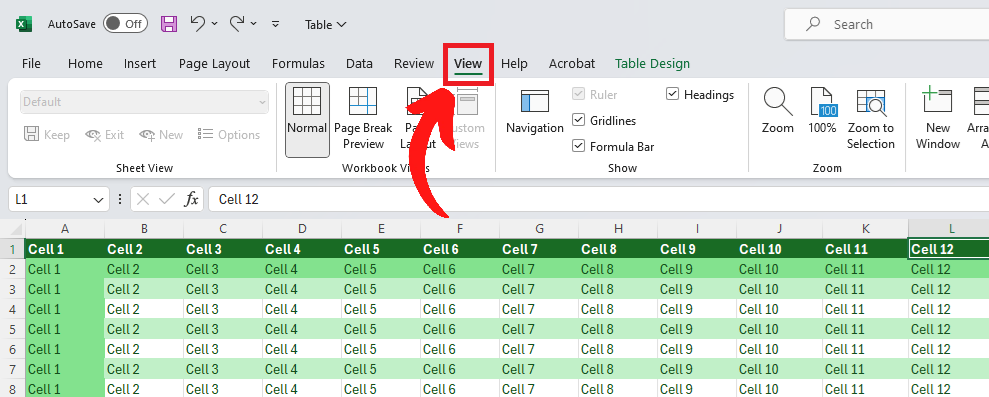
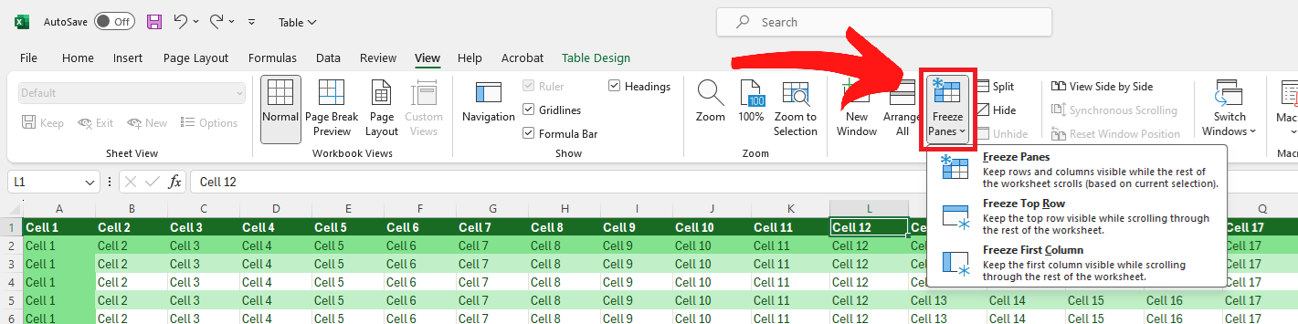
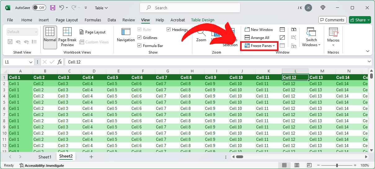
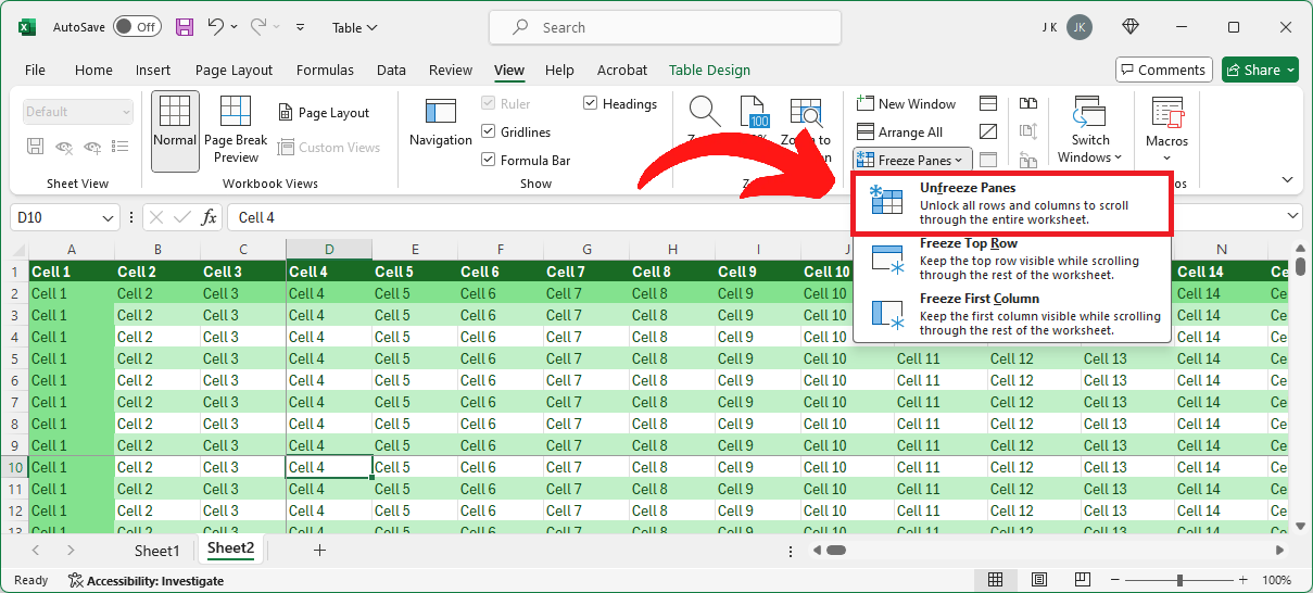
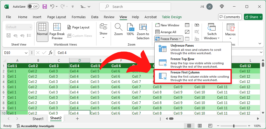
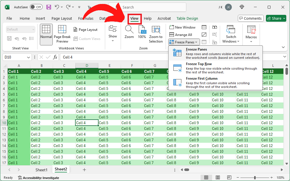
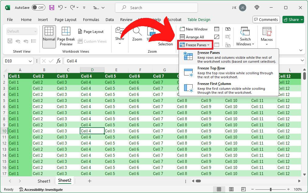
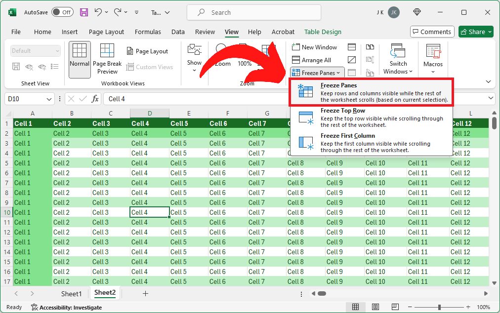
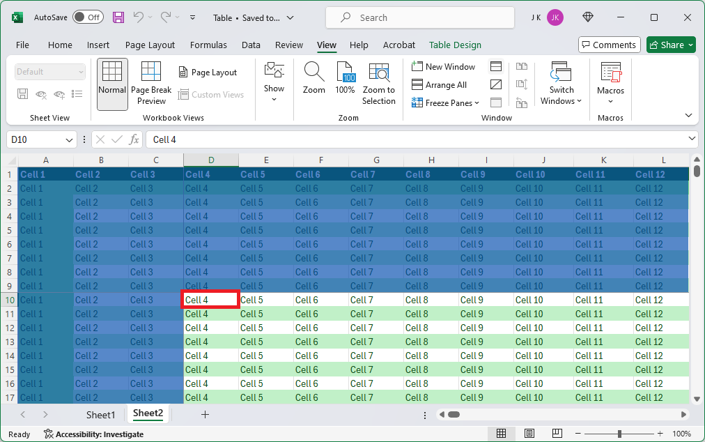
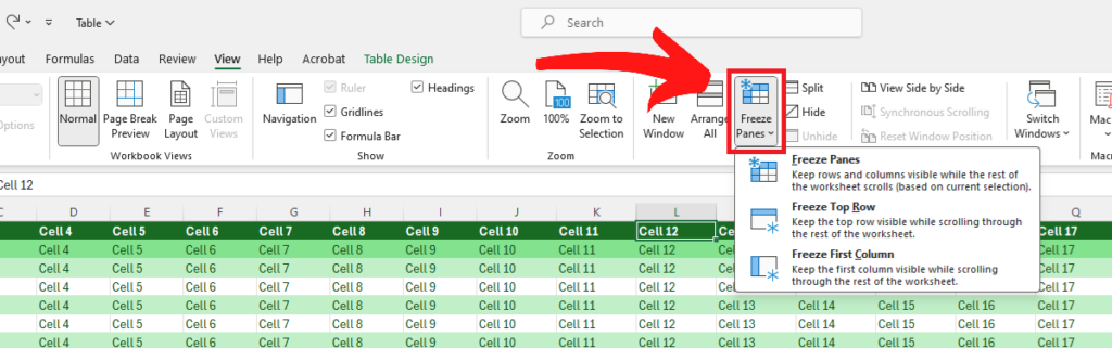
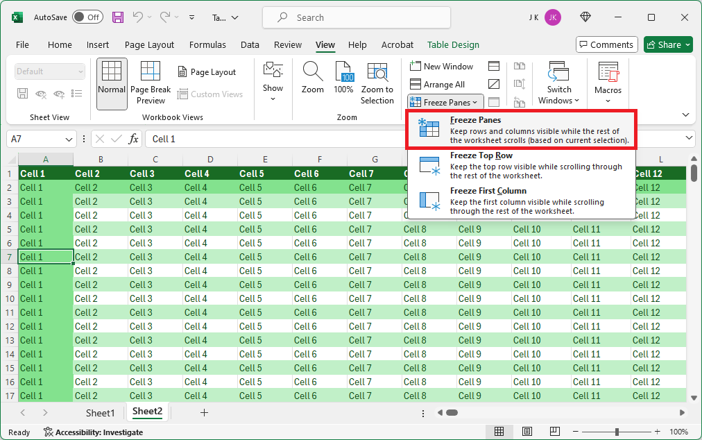
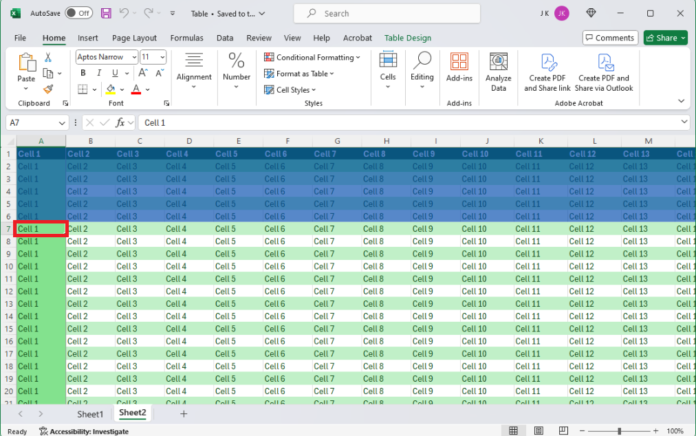
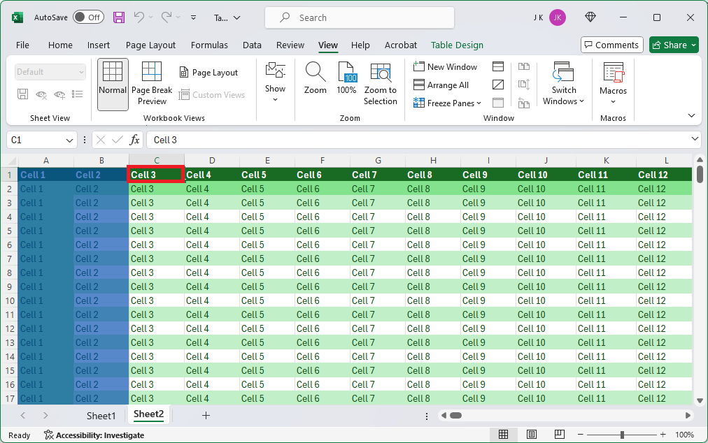
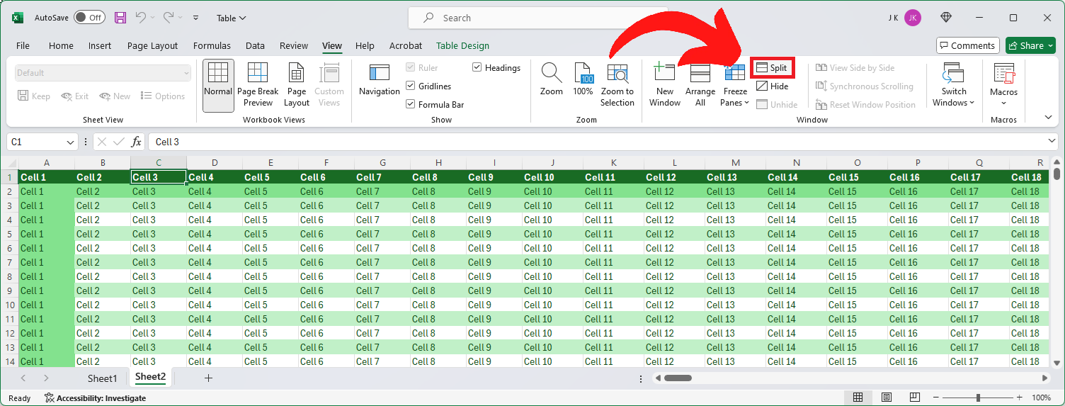
If parts of your spreadsheet are staying fixed in place as you scroll, those rows or columns are probably “frozen”. To unfreeze any rows or columns in your Excel spreadsheet, simply click on “View”, above the options ribbon, and then click on “Freeze Panes”, and then “Unfreeze Panes”. This will remove the frozen panes effect, so no rows or columns are frozen.

Request a Tutorial

What’s happening in the Excel community?

Excel

Experts

Excel Tutorials and Lessons